Hybrid Lattice Boltzmann Method (HLBM)

What is HLBM?

The Hybrid Lattice Boltzmann method is a method that not only yields dynamic visual effects, but is simultaneously more efficient, thus less computationally expensive without a greater space requirement. The hybrid lattice Boltzmann method, or HLBM, is a hybrid method the of particle level set method (PLSM) and the lattice Boltzmann method (LBM); thus, HLBM fuses the advantage of PLSM, which is realism, and of LBM, which is speed. HLBM refines the details gas and liquid behaviour, as they interact with each other and their surroundings. In addition, more "splashy" and dynamic visual effects can be achieved.

About the HBL method

To understand the approach taken when using HLBM, it helps to understand the approach of the methods it is derived from.

LBM

This method allows first order discretization of the Boltzmann equation. The Boltzmann equation is used to calculate gas behaviour on a microscopic scale. The lattice Boltzmann method takes an Eurlerian approach by dividing the simulation region into Cartesian grid cells, each only interacting with directly neighbouring cells. This is a relatively simple and fast method but this speed is achieved through the storage of distribution functions of neighbouring cells; this incurs a high memory cost. 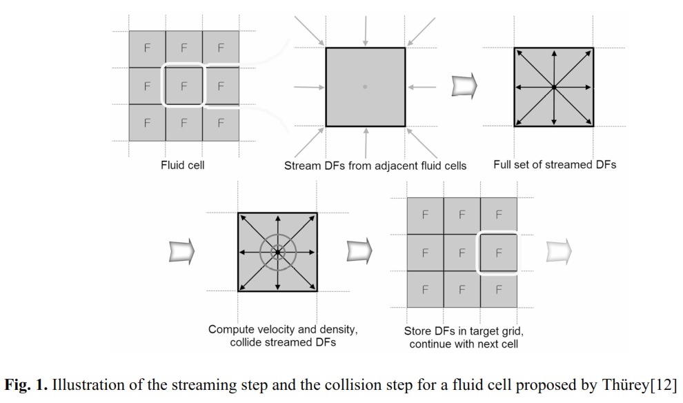The algorithm can be divided into two main steps, streaming and collision.
The equation for the streaming step is

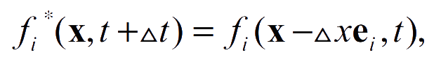
Δx is the cell size and Δt is the time step. This equation calculates the bulk flow and movement of the fluid.
The equation for the collision step is

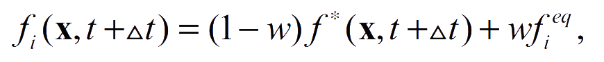
w stores the viscosity and f_ieq is the equilibrium distribution function that represents the stationary fluid. The result of these distribution functions is stored in an array. Each cell has 2 arrays for its neighbouring cells' last and current step. This part of the algorithm refines the streaming, by calculating the effect on the velocity of a particle due to collisions with adjacent particles. Thought streaming is refined, LBM still restricts the number of directions a particle may move.


To model the interaction between solids and liquids the no-slip boundary condition is used. This condition states viscous fluids with have a velocity of zero at solid boundaries and assumes liquids adhere to them. A boundary is placed half way between the fluid and obstacles cells. Thus if a neighbouring cell located at (x + Δte_i) is an obstacle while the current cell is streaming, the distribution function of the inverse direction is used.
f_i*(x, t + Δt) = f_`i(x,t)
`i denotes the value of the inverse direction of of a value with the subscript i.
In addition, regions that contain fluids are denoted with a flag. The distribution function of cells with empty flags are ignored. However, fluids may flow into these cells if they are not boundary (or obstacles). To keep track of this, another cell type is used, known as the interface cell. They form a closed layer between fluid and empty cells and the cell mass is used to update its type for the next time step.

LSM & PLSM

The level set implicitly constructs the surface between given fluids. The level set method discretizes Navier-Stokes' equations (NSEs and tracks the interfaces during simulation). The NSE for incompressible fluids is
∇⋅u = 0, continuity equation - the velocity of incompressible fluids is non-divergent
momentum conservation equation terms are: advection, diffusion, pressure, and external forces. To eliminate divergence, the Poisson equation must be solved with the Neumann boundary condition; this process incurs a large computational cost.
The level set function's evolution is described by this equation
ᶲ_t + u⋅∇ᶲ
Smooth surfaces are achieved through the nature of the level set function, but the liquid volume decreases dramatically during simulation.

PLSM overcomes the loss of volume in LSM, through the use of massless marker particles that assist with tracking flow characteristics in under-resolved regions around the interface.Label particles as positive or negative based on level set values. Positive particles are in the band near the interface with positive level set values and negative particles are near those with negative level set values These particles work to correct errors in the level set functions by comparing the level set functions from escaped particles and rid points.

The Algorithm

1. Run execute the LBM solver: where streaming and collision steps are performed, use Eq 1 and 2, respectively. Obstacle and free surface boundary conditions are applied, and the distribution function of next time step, f_i(x, t + Δt), for each lattice is calculated

2. Calculate the macroscopic velocities for the current time step, u(x, t), use ρ = Σf_i, and u = Σe_i * f_i Eq 4

3. Extrapolate the velocity field, u(x,t), to the gas region. u_ext(x,t) This allows advection of PLSM

4. Advect the level set function, ᶲ(x,t), and particles, p_k(t), by the extrapolated velocity field, from step 3.

5. Correct errors of the level set function with advected particles in PLSM

6. Calculate 2 different density fields obtained from LBM and PLSM solvers.

7. LBM part: density of each cell, ρ_LB, is calculated with multi-resolution density calculation scheme up to 3rd level as described in Table 1. Fig2 shows 2D example of density calculation method. Add density difference between LBM and PLSM solvers to distribution functions to correct the LBM errors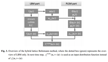

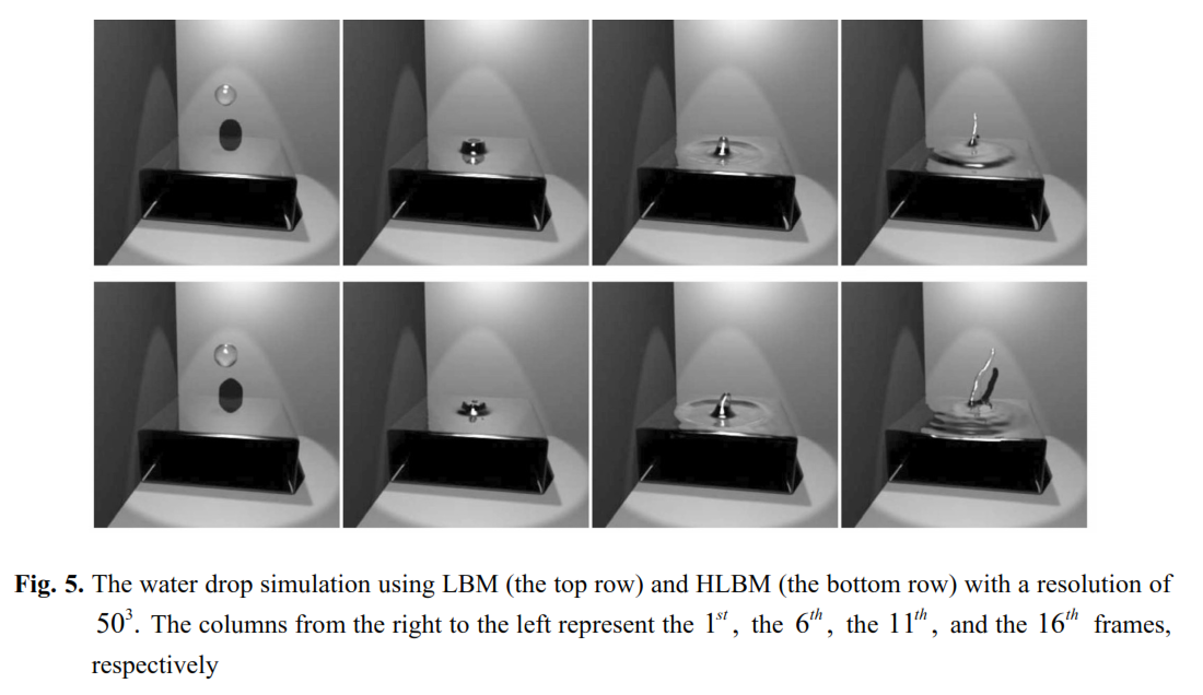
Below is the HLBM (bottom) simulation juxtaposed with the LBM (top).